
Main Page |
Using time domain measurement
|
 We can measure all those factors using a TEF but we can't easily generate the test tone required by the TEF by
directly stimulating an actor, at least not comfortably and within union rules. A reasonably accurate substitute test source must be found,
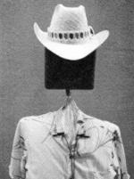
preferably one that doesn't have an agent. The test dummy (complete with cowboy hat and loud Hawaiian shirt) was
nicknamed Leroy. He consists of a small speaker enclosure, with a 5 inch loudspeaker, mounted on a microphone stand, with a pillow to simulate the torso surface area (if not exactly its density) and wrapped in a shirt to provide lapels for attaching
microphones to. Small speakers, such as the one in use here, have similar directional characteristics to the human
voice, providing a convenient method of examining the pickup characteristics without involving live actors.
We can measure all those factors using a TEF but we can't easily generate the test tone required by the TEF by
directly stimulating an actor, at least not comfortably and within union rules. A reasonably accurate substitute test source must be found,
preferably one that doesn't have an agent. The test dummy (complete with cowboy hat and loud Hawaiian shirt) was
nicknamed Leroy. He consists of a small speaker enclosure, with a 5 inch loudspeaker, mounted on a microphone stand, with a pillow to simulate the torso surface area (if not exactly its density) and wrapped in a shirt to provide lapels for attaching
microphones to. Small speakers, such as the one in use here, have similar directional characteristics to the human
voice, providing a convenient method of examining the pickup characteristics without involving live actors.
 Standing pickup        Seated at a Desk     Automobile Front Seat       |
The TEF analyzer is a very convenient tool for looking at these characteristics. To see what information it will give us, three test examples are presented. The first is with the test source in a small warehouse environment with concrete floor and walls, steel roof trusses and roof deck and many diffuse surfaces. Measurements were made using a short shotgun microphone, an omni lavalier and a cardioid lavalier. The second example has the test source in a seated position at an office desk, with office dividers present and typical acoustical tile ceiling overhead. Measured here using the shotgun, two lavaliers and a PZM. The third example has the test source in the driver's seat of a small automobile, measured using two lavaliers and a PZM microphone.
The first example is shown in Fig 2, here the short shotgun is approximately I metre above the test source (without the hat), typical of a boom' pickup. The cursor (the crosshairs) on the display marks the arrival of the direct sound. The levels of the direct arrivals, early reflections and the major reflection from the floor can be read directly from the display. The room is technically too small to have a reverberant field, it is actually a dense field of reflections and the fairly regular spacing of them can be seen.
Fig 3 shows another handy feature of the TEF program. In the TEF software TEF 2.0, the E cursor program allows you to do an RT60 measurement, actually measuring the reverb as 'heard' by that microphone position. The sloping line is the Schroeder Integration Curve, which defines the amount of energy contained in the sound field. If you remember any calculus, here is a real world application for it, luckily it is all done by the TEF. By locating two points on the integration line in the reverberant field, the TEF will calculate the slope of the line connecting them and determine the RT60. Ideally you would want at least 10 dB of level difference between the two points to ensure accuracy. The downward curvature of the line, just past our second RT60 point, does not indicate that the reverberant field suddenly disappears. What it means is, to get an accurate picture of the reverberant field right to the edge of the display, we would require a slower sweep rate. The one chosen did not allow time for all the energy in the sweep to get back to the microphone. By slowing the sweep rate from 1000 Hz to 500 Hz in this example we could have obtained more data on the right side of the display. In this case, our primary interest is in the early arrivals, and having a quick sweep. You can check your two reverb calculation points for curve fitting by using the 'D' command, which draws the regression line shown.
In Fig 4, we have installed the cowboy hat. You can see the direct sound is a couple of dB lower in level. There are some changes in the early arrivals, from refraction and diffraction around the hat. You can see that there are a couple of arrivals close to the direct sound that have increased in level and the reflection from the floor is a bit broader in time.
In Fig 5, the test source, sans hat, is in the same position but we have switched to an omni lavalier microphone. You can see a major difference in the early arrivals, they are all much lower in level when compared to the direct signal. Also note the difference in density of the reverberant field. Much of the pickup of the reflection is being blocked by the torso.
Now in Fig 6, Leroy is wearing his hat again and you can see two distinct arrivals very close together, one a reflection from the hat brim. To see the effect of this second arrival, look at Fig 7. Here you can see the notch created by cancellation at approximately 2800 Hz and the bump at 2100 Hz. You can expect the location of the notches to change with hat position too. If the actor pushes his hat back that will sweep the filter down.
In Fig 8 we doff our hat and use the cardioid lavalier. There is an increase in the direct sound pickup and a substantial reduction of early arrivals is apparent, The initial portion of the reverberant field is less dense as well. It is picking up reflections from the ceiling area now, which do not seem to decay as fast as those picked up with the omni. This would still be audibly interpreted as a very 'dry' pickup, with very little room character.
The second example is one that would crop up regularly in office scenes, dinner table scenes, restaurants and so on. In Fig 9, we have the office desk position, this time using the omni lavalier for pickup. The direct sound has only 14 dB advantage over the first group of reflections Note that the bulk of the energy arrives in the first 20 ms and the decay is rather fast. This is quite a dead space. All these early arrivals will play havoc with the frequency response just like the cowboy hat did. And they will change with the actor's position.
Fig 10 shows the cardioid lavalier and its attendant drop in early reflection pickup, Oddly enough it has a higher level in the late arrivals but they are more diffuse and spread over a greater time. Fig 11 shows the PZM on the desk surface, overall its pickup looks like the omni lavalier but with a lower, more uniform level of early arrivals spread over a greater time, Fig 12 shows the short shotgun pickup, again approximately 1 metre overhead. A substantial change in the direct to reverberant energy is visible, with barely 12 dB of advantage for the direct sound. The greater reverberant field would make this a very 'distant' pickup,
The third example, the front seat of an automobile, required changing the band of frequencies swept by the TEF. This changes the total display width from 82 ms to 26 ms. This allows more detail of the early arrivals to be seen, an important concern since all the surfaces are so close. The time domain and frequency domain are inverses of each other, so as you acquire more time resolution, you lose frequency resolution and vice versa. In this case, broadening our frequency content has shortened the time scale of the display. At the 1 kHz sweep rate, this raised the total sweep time from 5 to 15 sec.
The omni lavalier used in Fig 13 shows a very high level of reflected energy due to all the hard surfaces close to the source. The omni lavalier produces a pickup with a very even decay, even though the decay is incredibly short, as shown in Fig 14. All the arrivals of any significant level in the front seat of an automobile will have more impact on response than on perceived reflections All the reflective surfaces are a few inches to a few feet away. The notches created in the pickup itself cannot be fixed through equalization since they are the result of phase cancellation at the microphone diaphragm, there is no sound left to equalize.
Fig 15 is the same test source with a cardioid lavalier. A strong reflection from the roof and windshield is visible, and you might expect this will cause some response irregularities. Fig 16 shows the of a PZM on the seat between driver and passenger. The direct signal is actually lower in level than the combined reflections that arrive 2 ms later, there are a lot of reflective surfaces in an automobile. Fig 17 again shows the PZM but this time on top of the instrument panel, close to the base of the windshield. We have a much higher direct arrival and the early arrivals are bunched closer together but the effect of spreading them over almost 2 ms is, we look at. the resultant response in Fig 18. It makes you wonder why you spent all that money on a flat response microphone.
When performing ETCs where you need to measure very long reverb times in large rooms, you will run into conflict. If
you actually display a full 6 sec (6,000,000 microseconds) on the screen, you will lose detail in the early arrivals that are most
critical for dialogue replacement work. In these instances, two sweeps would be made, one to cover the long period far RT60
measurements and- one with a short time period to measure early arrivals in detail. As long as you keep the swept
frequencies in the voice range, you will get relevant data.
When it becomes necessary to look at frequency response, you can limit the bandwidth to the voice range,
approximately 150 Hz to 5 kHz. In the frequency response displays in these examples, the resolution was chosen to
be 100 Hz, allowing the display of major comb filtering and the use of a relatively fast sweep rate of 1 kHz. It would
be possible to get a frequency resolution of approximately 32 Hz with this sweep rate but the additional detail can be
distracting as it begins to show variations that will change with the actor's head position, his arms, eyeglasses and
other minor, short term influences.
Once you know the approximate distance
around the actor in which the action will occur, you can optimize the bandwidth setting. By choosing the optimum
bandwidth you can select the size of the 'sphere of interest' around the actor. Along with resolution information the
bandwidth specification will give a distance in feet. This describes the total pathlength from the test speaker to the
microphone that will be accepted by the TEE In the usual application of TDS measurement, this describes the
measurement ellipse (see Fig 19). If you took a string of the length given, tied one end to the speaker and one end to
the microphone, any point you could stretch the string to would be on the surface of the ellipse. With the source and
the receiver so close to each other, as on our test dummy, the ellipse is nearly spherical (see Fig 20).  If you choose a
bandwidth that gives a distance of 32 ft, the measurement will include all sound paths within a sphere of 16 ft radius
about the actor. If you choose a bandwidth that gives you a distance of 2 ft, the measurement will include all sound
paths within a 1 ft radius.
If you choose a
bandwidth that gives a distance of 32 ft, the measurement will include all sound paths within a sphere of 16 ft radius
about the actor. If you choose a bandwidth that gives you a distance of 2 ft, the measurement will include all sound
paths within a 1 ft radius.
The application of the TEF in film and TV sound has to begin on location. Once a microphone technique for a given scene has been chosen, a test dummy similar to Leroy would be placed on the set, equipped with the same type of microphone and wardrobe as the actors will have. A test sweep would be done and stored. If there were a number of locations on the set where dialogue would take place, especially if some of those locations will have different acoustical characteristics, a number of test sweeps may be required. The sweeps only take a few seconds each, and since the TEF does not require silence to work in, it would be done while cameras and lights are being prepared-long before the director would start tearing his hair out about delays.
The new TEF 12 Plus is especially useful here, due to its faster operating system, giving quicker access to various command menus. The equipment could be streamlined by using a powered speaker for Leroy's head and it could be attached to a mannequin torso to provide an easier-to-handle assembly. At the end of the shoot the disk containing the data could be kept with the audio tape from the shoot and so travel together to the audio-post house for appropriate changes and additions.
The TEF has other applications here as well. By augmenting the ear, the TV and film sound person could fine tune microphone technique. By listening to, then measuring, various pickup techniques, troubleshooting certain pickup problems can be done quickly and accurately. You could take a detailed look at the comb filtering that occurs when two actors with lavalier mics approach to within a few inches of each other. A catalogue of typical pickup methods could be made and then stored in memory in digital delay/reverb units. This would be applicable for a TV show that used a number of standard sets on a sound stage. The TEF can be used to measure the combined equalizer/delay/reverb electronic chain, to view its time response and frequency response. Hundreds of aspects of microphone technique could be examined in detail, from the effects of microphone position to the effects of cowboy hats as shown here.
There is no reason to stop at dialogue replacement, virtually the entire post processing chain is TEF'able, starting in the voiceover studio, right through to the tape recorders. The TEF can be the audio lie detector, usable anywhere a two-port measurement can be devised.
While the cost of a TEF 12 Plus may seem high for a single box of equipment that does not directly produce
revenue, it can reduce time spent on many types of projects and increase accuracy. It costs about the same as a
good synchronizer and could smooth post-production work as effectively. Its applications are limited by the
imagination and need of the user; those seem like minimal limitations in the recording industry.
![]()